To make a spring with Geometry Nodes in Blender, all we need to do is use some vector math. Taking a straight line as a basis, we can move its points in accordance with the circle equation so that in the end they form a spring.
 .blend file on Patreon
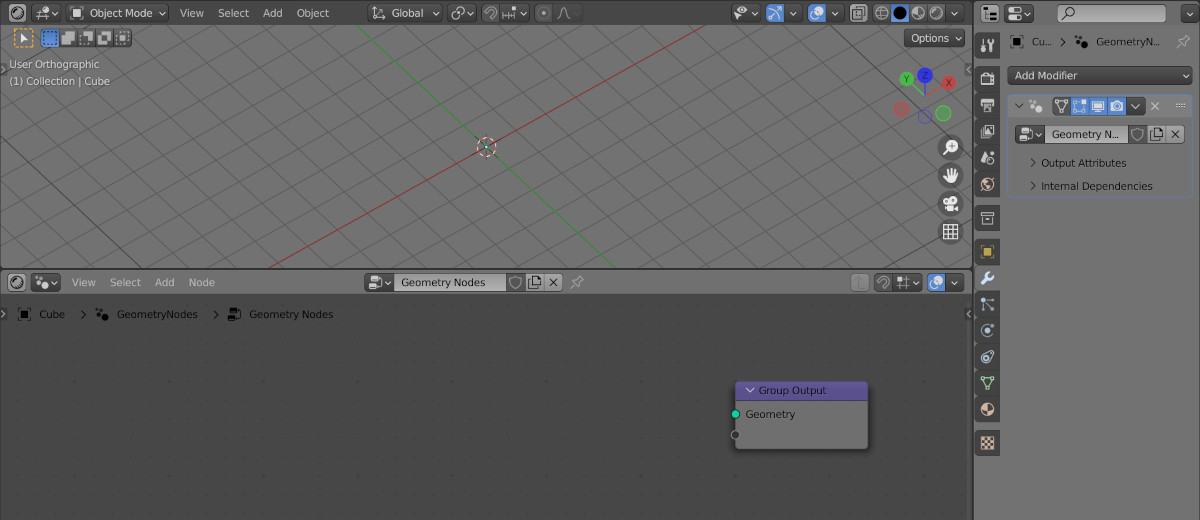
Let’s open an empty scene in Blender, add a cube to it (shift+a – Mesh – Cube), append a Geometry Nodes modifier to it, and by pressing the “New” button create an empty Geometry Nodes tree.
Delete the Group Input node since we won’t use the original cube geometry, but build the spring from scratch.
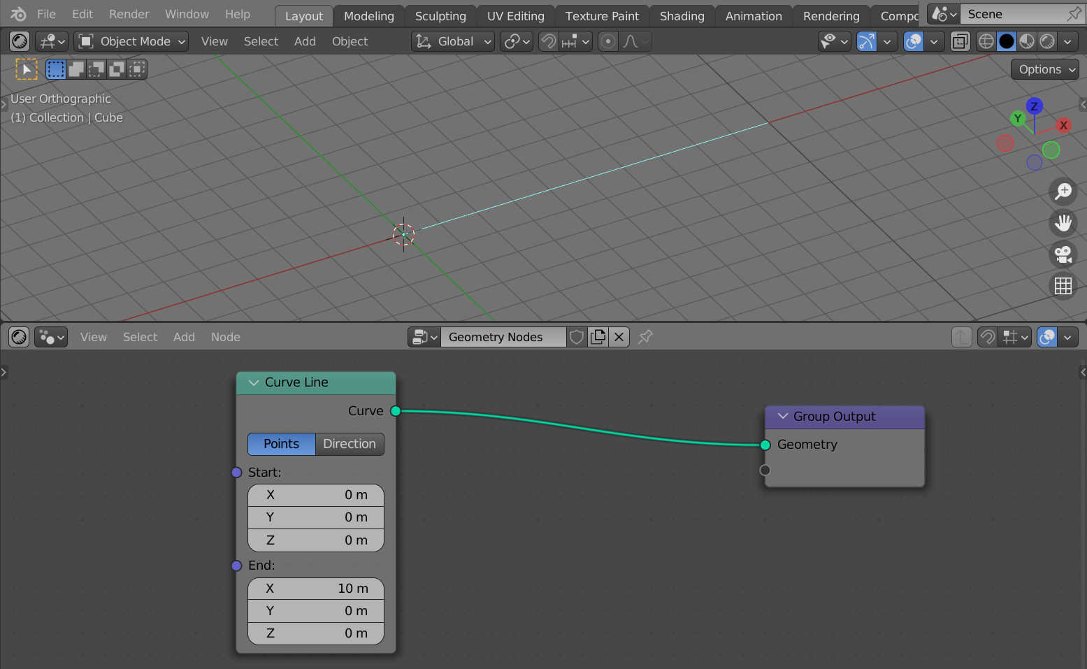
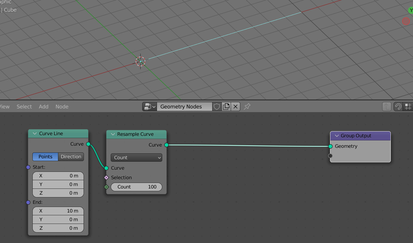
Add a Curve Line node (shift + a – Curve Primitives – Curve Line). This node creates a straight line consisting of two points. Set the location of the first of them at the origin of coordinates – set all the coordinates of the Start point field equal to 0.0. Place the second point at a distance of 10 meters along the X axis – the X coordinate at the End point field set equal to 10.0, and the rest – 0.0.
Link the node to the Group Output node.
Let’s subdivide the curve by adding intermediate points to it. To do this, add a Resample Curve node to the tree (shift + a – Curve – Resample Curve) and set the number of points to 100.
Now for some math.
To get a spring from a line, we need to move each of its points so that it lies on a cylinder whose axis coincides with our line.
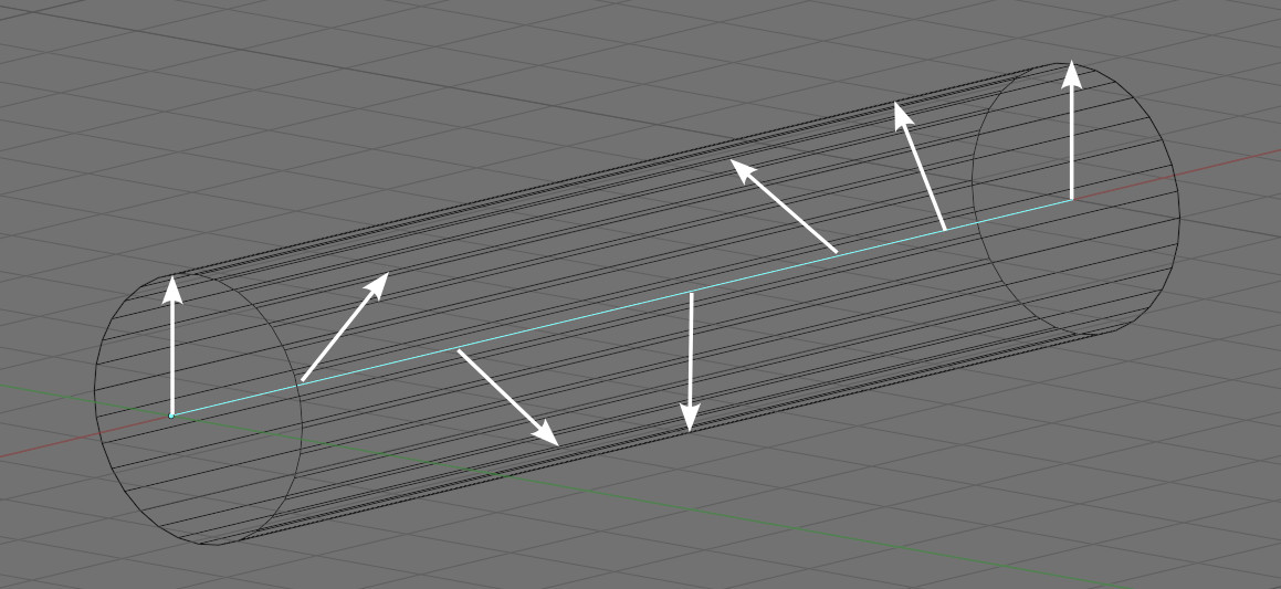
Since the cylinder is a circle stretched along our line, we can use the circle equation to calculate how much we need to offset the points.
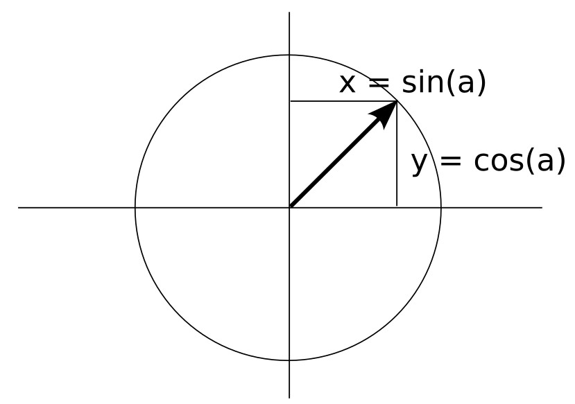
As we know, the X and Y coordinates of points on the circle are determined depending on the angle of inclination of the “a” vector, which in our case of the circle translation along the straight line directly depends on the current position of the point on our line.
Let’s get back to our nodes.
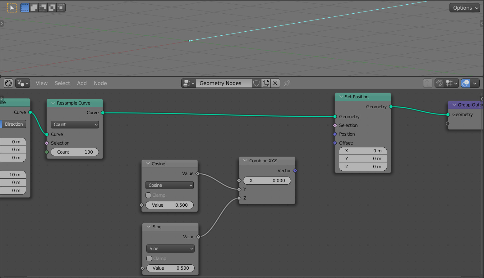
To move the points of the line in the required way, add the Set Position node (shift+a – Geometry – Set Position) to the main branch of the node tree.

We need to link the point offset to its Offset input. This input has the vector type.
Let’s implement the circle equation using nodes.
Add a Combine XYZ node (shift + a – Vector – Combine XYZ).
Since our follows the X axis, if we look at it from the end (so that the cylinder looks like a circle), the Z axis will correspond to the Y axis from the equation and the Y axis – to the X axis from the equation.
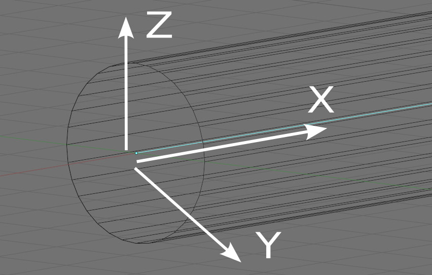
Therefore, the equation must be assembled by linking sin() and cos() with the Y and Z inputs of the Combine XYZ node.
Add a Math node (shift + a – Utilities – Math), switch it to the “sin” mode, and link its Value output to the Z input of the Combine XYZ node.
Add another similar Math node, switch it to the “cosine” mode and link it with the Y input of the Combine XYZ node.
Now we need to associate the circle equation with the coordinates of the points on the line.
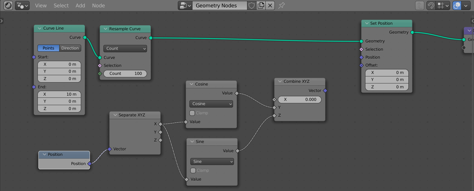
Add a Position node (shift + a – Input – Position). This node returns the position vector of each point on the line.
Since the angle of rotation “a” depends only on the distance of the point from the beginning of the line, then we need only their X coordinate from the position of the points.
Add a Separate XYZ node (shift + a – Vector – Separate XYZ) and link its Vector input with the Position output of the Position node. Link the X output of the Separate XYZ node with the Value inputs of both Math nodes.
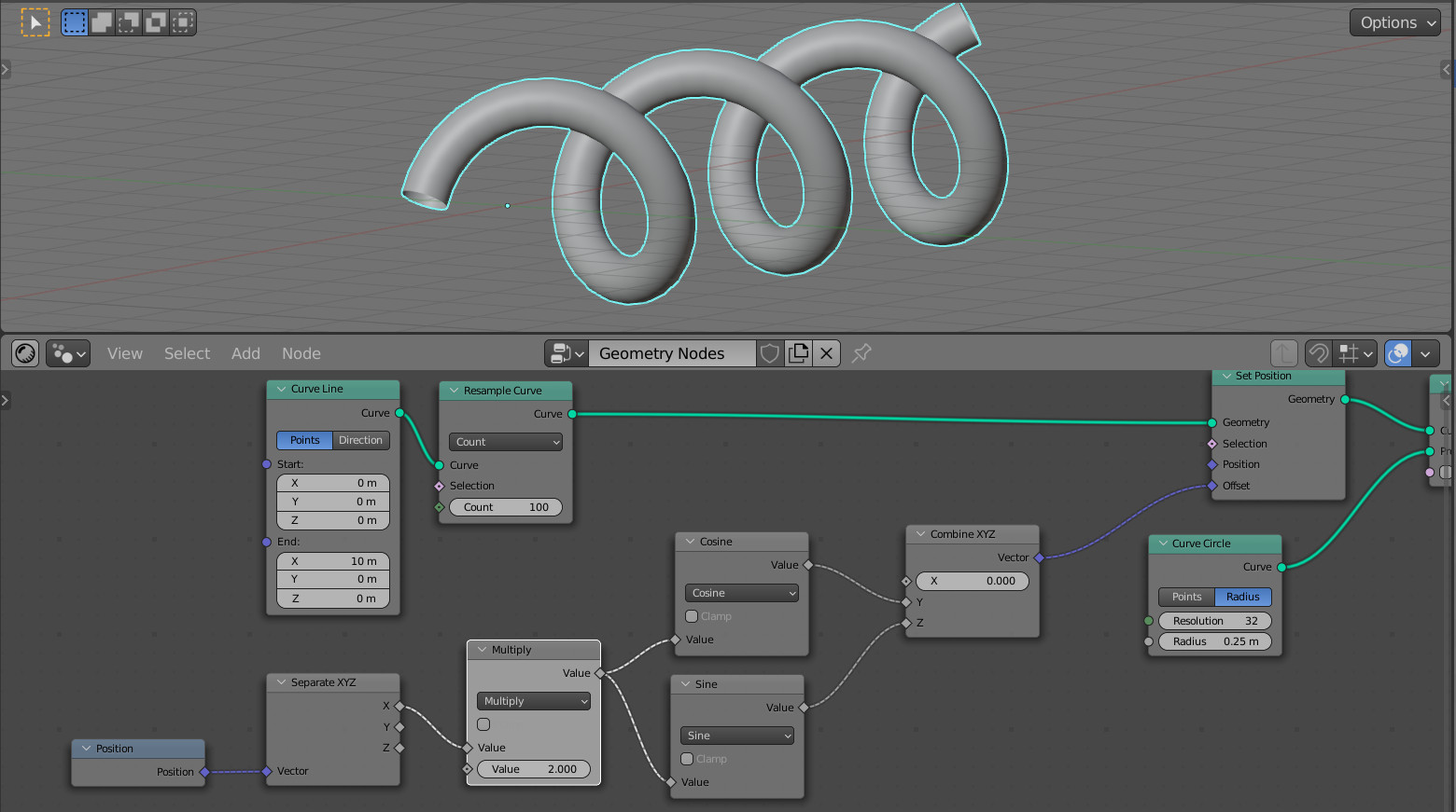
We got the offset of each point of the line to the circle. Link the Vector output of the Combine XYZ node with the Offset input of the Set Position node to give the points of the line a calculated offset.
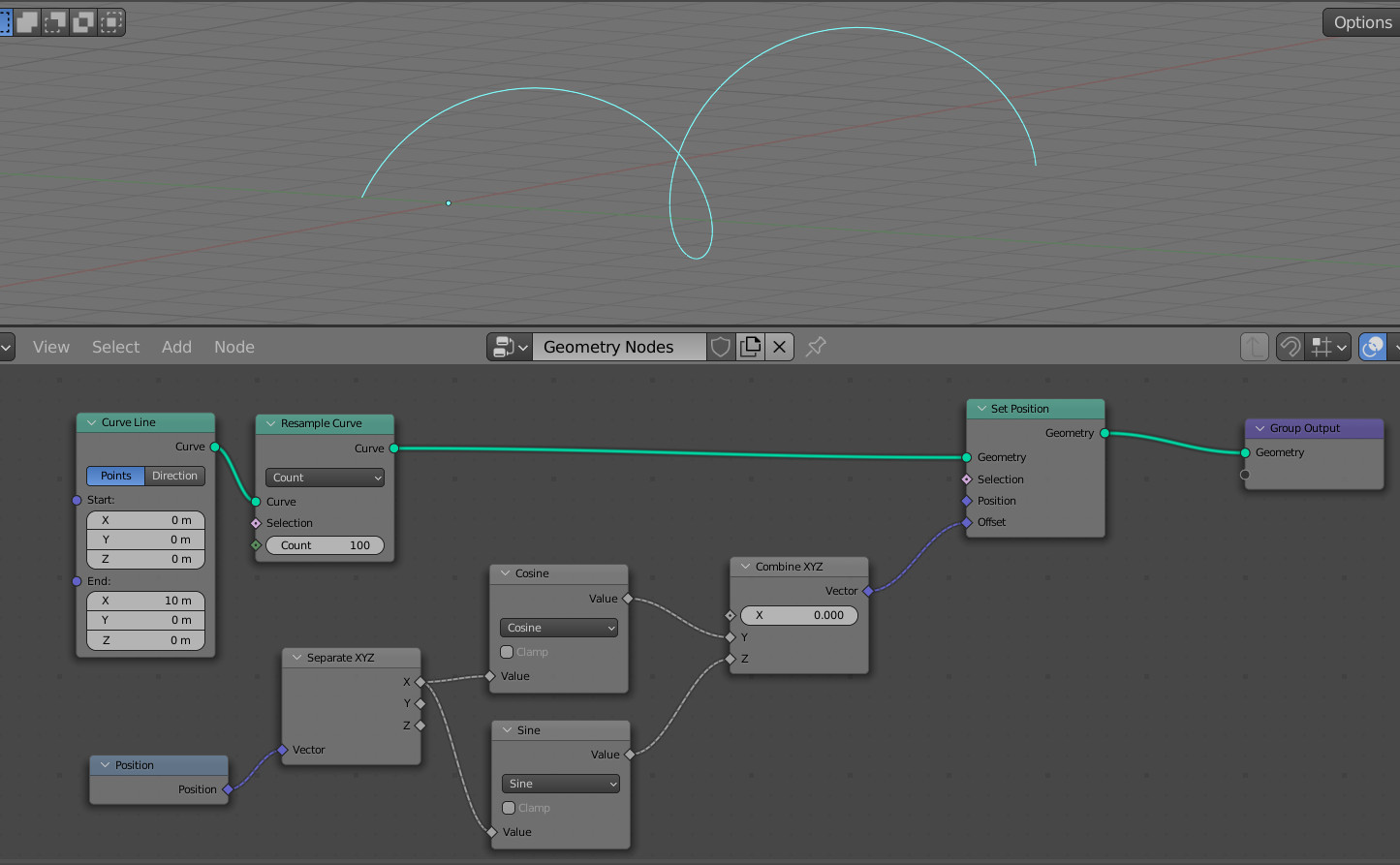
The straight line has become a spiral spring.
To give it thickness, add a Curve To Mesh node (shift + a – Curve – Curve To Mesh) to the main branch of the node tree, after the Set Position node.
Also add a Curve Circle node (shift + a – Curve Primitives – Curve Circle). This node will set a profile that bypasses our spring, giving it thickness. Link its Curve output with the Profile Curve input of the Curve To Mesh node.
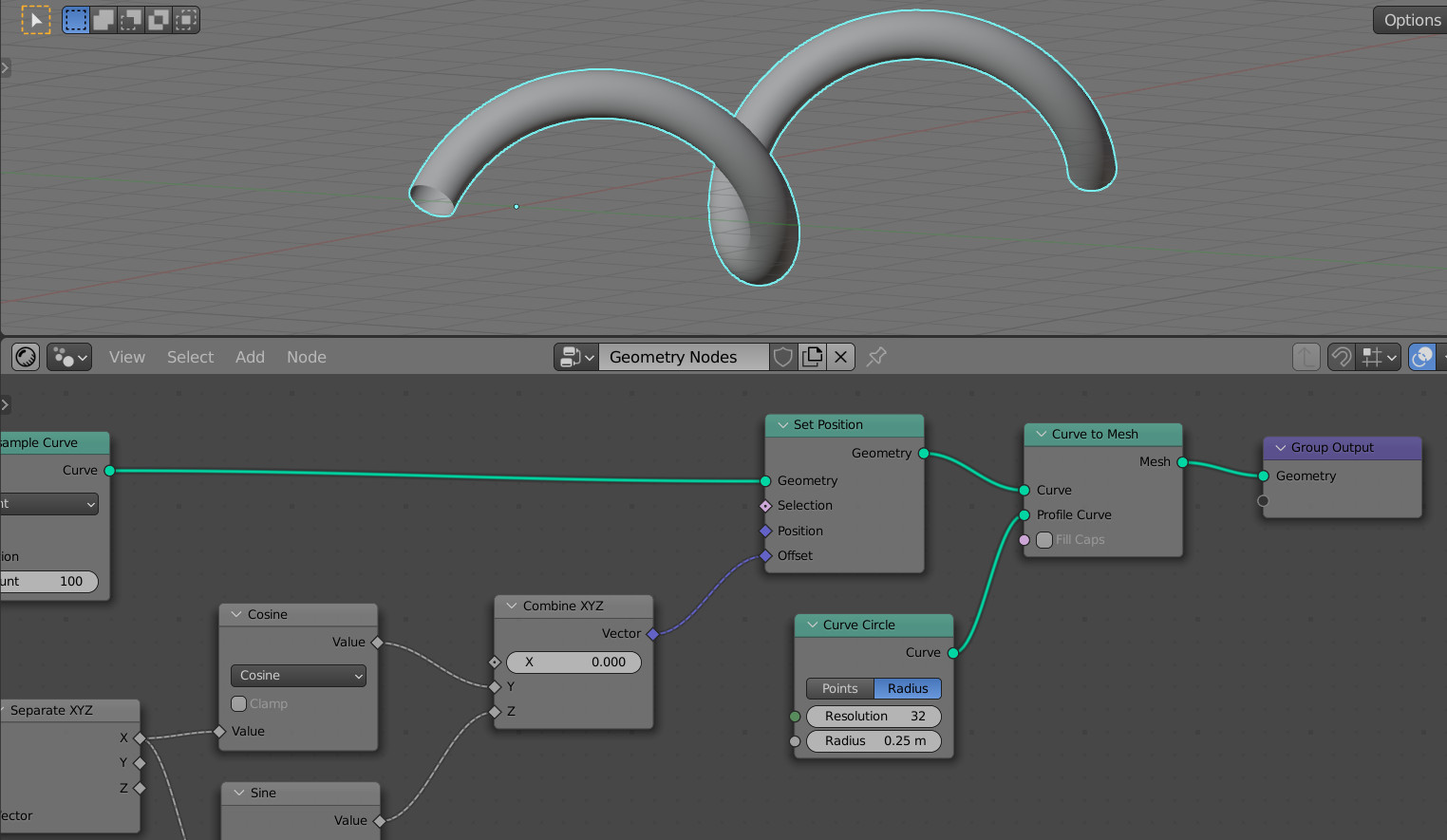
Set the value of the Radius field to 0.25. By changing the value of this field, we can dynamically change the thickness of the spring.
To control the number of turns of the spring along its length, we just need to add a coefficient when calculating the angle “a” in our equation for offsetting points along the circle.
Add a Math node (shift + a – Utilities – Math), switch it to the Multiply mode and insert it into the equation calculation branch before the “sin” and “cosine” nodes. Set the node’s Value field to 2. By changing it, we can dynamically change the number of turns of our spring per unit length.
The more turns per unit length we set, the more angular spring we get. This is due to the fact that it lacks points to achieve smoothness.
To achieve smoothness, we can simply increase the number of points into which we subdivide the original line by increasing the value of the Count field of the Resample Curve node.
Or, while our line is of the Curve type, set the handle auto-detection to its points.
To do this, add a Set Spline Type node (shift + a – Curve – Set Spline Type) to the main branch of the tree and insert it before the Curve To Mesh node. Switch it to the Bezier mode. Add a Set Handle Type (shift + a – Curve – Set Handle Type), switch it to the Auto mode and insert it into the main branch of the tree after the Set Spline Type node.
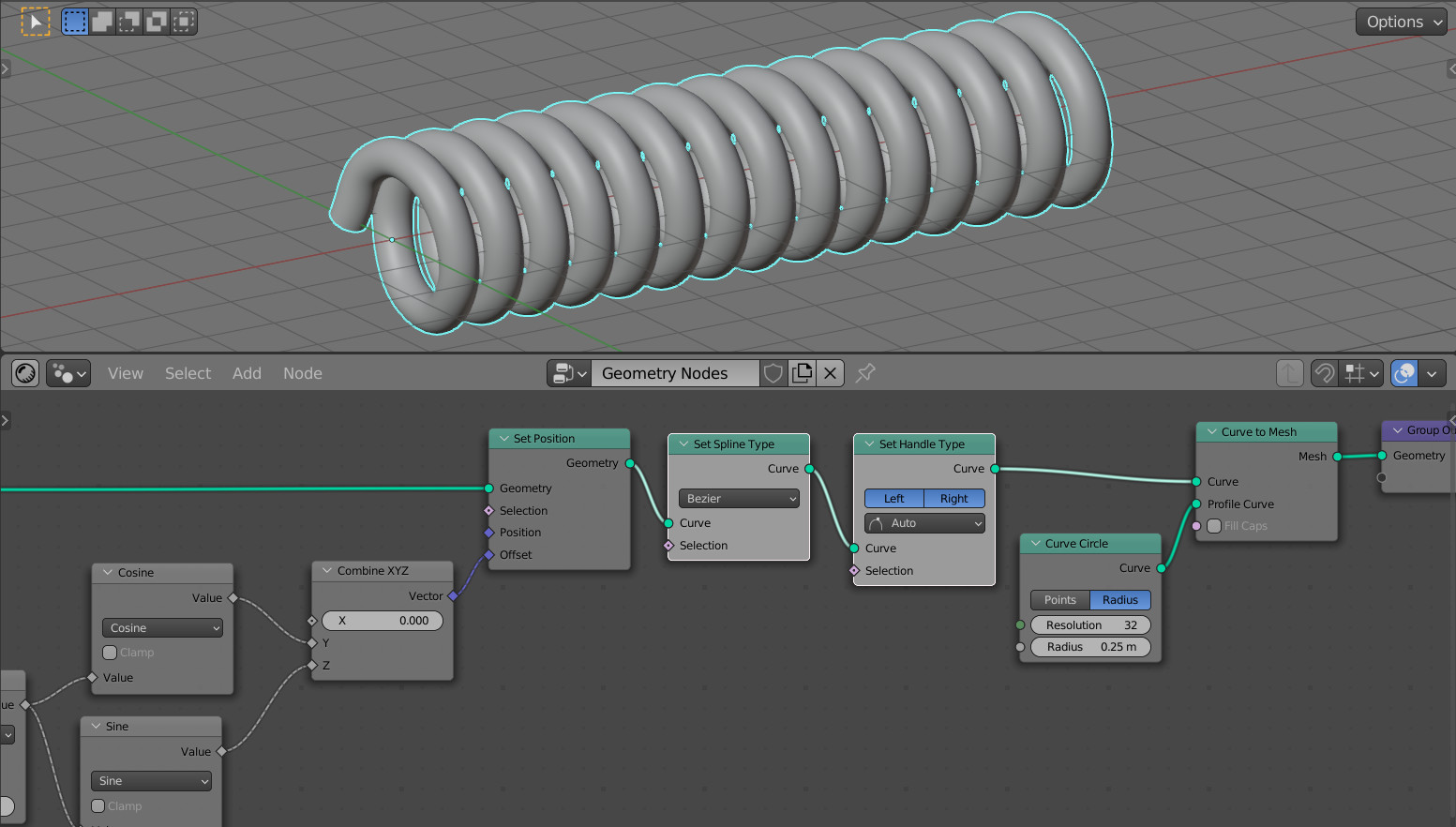
Now we can set a higher density for our spring without significantly increasing the number of points in its geometry.
To dynamically change the diameter of the spring, we just need to add a coefficient to our equation for calculating the points offset along the local X and Y axes.
Add a Math node (shift + a – Utilities – Math), switch it to the Multiply mode and insert it into the branch for calculating the points offset between the Sin and Combine XYZ nodes. Add exactly the same node to the branch between the Cosine and Combine XYZ nodes.
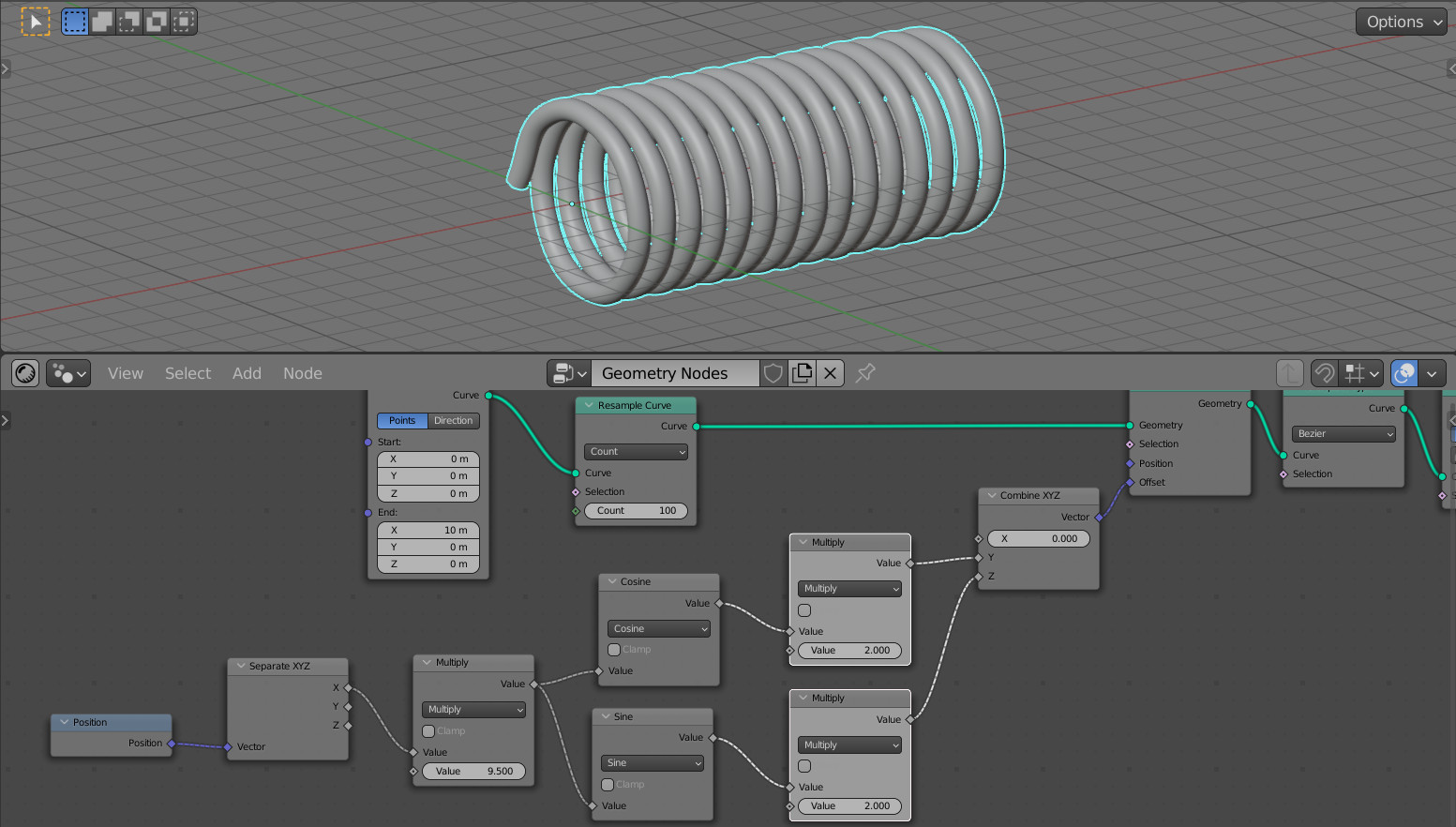
In both nodes, set the Value field to 2. By changing it, we can dynamically change the diameter of the spring.
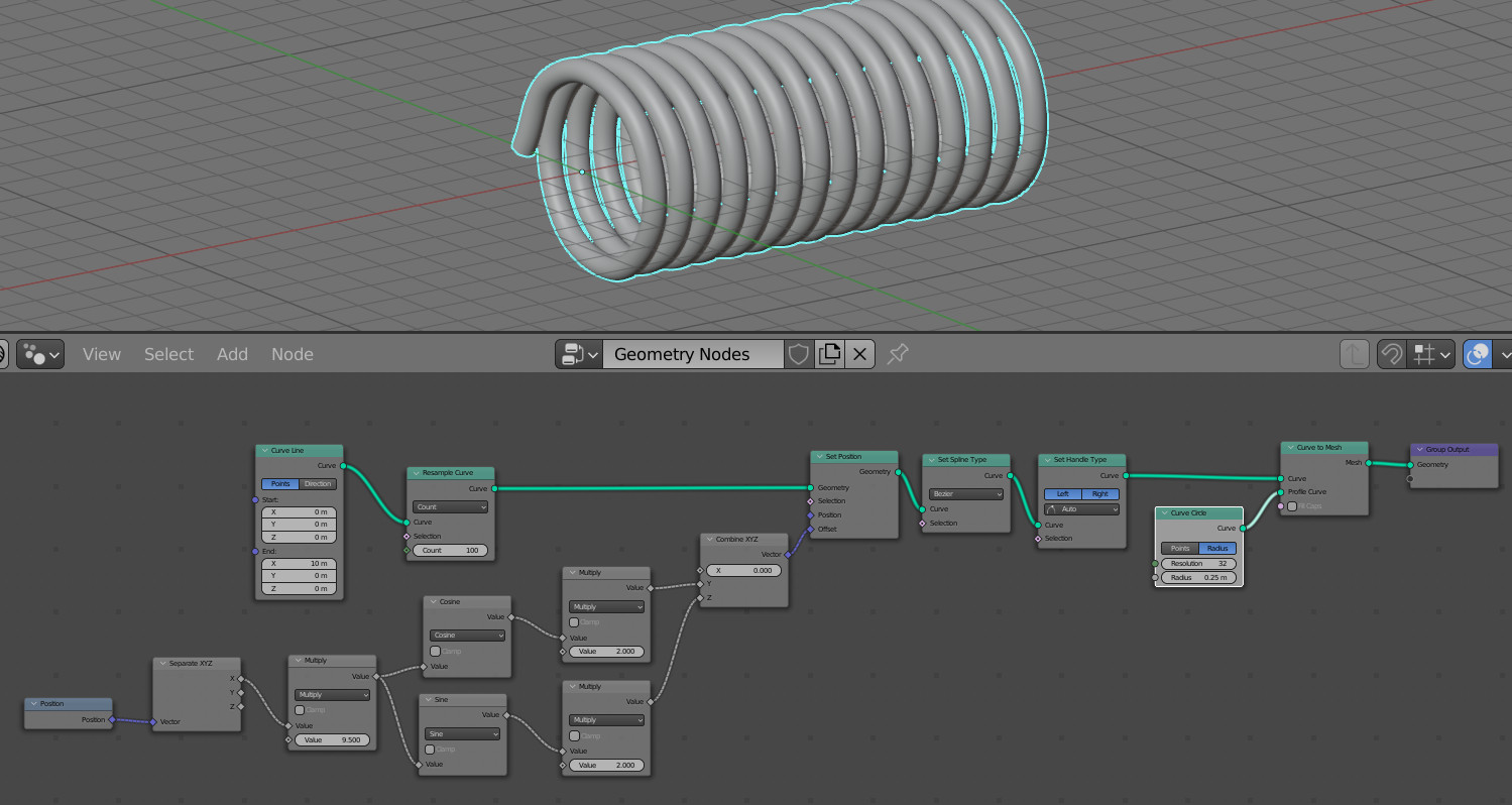
The final node tree: